PCA Tutorial
PCA of a MD trajectory
In this tutorial, we will be performing PCA on a MD trajectory of protein. Before doing the PCA, we need to prepare the trajectory which includes removing periodicity and removing water molecules. Most of the MD packages have options to do this. We will be using GROMACS in this tutorial. We will be using .xtc format for trajectory and .pdb for topology file. Any other common trajectory format should also work with MODE-TASK.
1. Preparation of trajectory
1.1. Remove periodicity
gmx_mpi trjconv -s md_01.tpr -f md_01.xtc -o md_01_noPBC.xtc -pbc mol -ur compact
select system to apply it.
1.2. Remove water
gmx_mpi trjconv -s md_01.tpr -f md_01_noPBC.xtc -o md_01_noWAT.xtc -n index
and select protein
2. Create a working directory
First, create a directory for all the MODE-TASK scripts using the Linux command:
mkdir ModeTask
Copy the entire contents of the MODE-TASK scripts into the MODE-TASK directory.
Within this directory create a folder called Tutorial:
cd ModeTask
mkdir Tutorial
We will run all scripts from the MODE-TASK directory. Move the trajectory (md_01_noWAT.xtc) and topology file (complex.pdb) into the Tutorial directory.
3. Running PCA
MODE-TASK includes tools to perform PCA on Cartesian coordinates as well as internal coordinates. It also allows users to run different variants of PCA on a single MD trajectory.
3.1. PCA on Cartesian coordinates
Run the following command to perform the singular value decomposition (SVD) PCA on CA atoms.
pca.py -t Tutorial/md_01_noWAT.xtc -p Tutorial/complex.pdb -ag CA -pt svd
Output:
(a)- Various output files are written to the out_md_01_noWAT.xtc directory. 2D Plot of first 3 PCs, Scree plot, RMSD plot, and RMSD Modes plot. For details about these output files, please refer to the MODE-TASK documentation.
(b)- Command line output: Following output is redirected to command line.
Results will be written in out_md_01_noWAT.xtc
Reading trajectory Tutorial/md_01_noWAT.xtc ...
No reference structure given, RMSD will be computed to the first frame in the trajectory
Trajectory info:
Total 101 frames read from Tutorial/md_01_noWAT.xtc
MD time is from 199000.0 to 200000.0 ps
13244 atoms and 861 residues in the trajectory
Atom group selected for PCA: CA
Total 860 CA atoms selected for analysis
KMO for input trajectory is 5.25051335835e-06
RMSD written to rmsd.agr
Performing SVD (Single Value Decomposition) PCA with 'auto' svd_solver
Trace of the covariance matrix is:  4.9427056479
cosine content of first PC= 0.777934456531
cosine content of second PC= 0.643848137376
cosine content of 3rd PC= 0.70061477062
cosine content of 4th PC= 0.530112237076
3.2. Visualizing the results
2D Plot of the first 3 PCs in grace and png format is written. In order to open the .agr file with xmgrace run the following command.
xmgrace out_pca_test_trj.xtc/pca_projection1_2.agr
You can also visualize the .png format figure plot by opening it with your favorite picture visualizer. In the same way, open the rmsd.agr and pca_variance.agr.
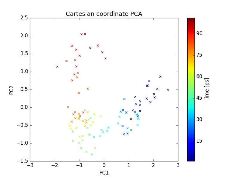
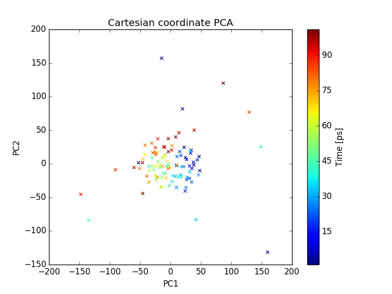
plot of PC1 and PC2
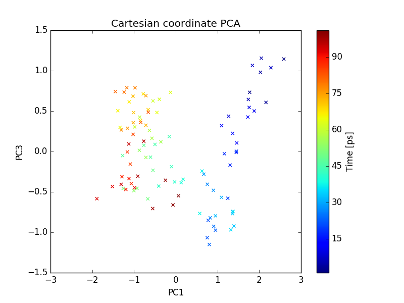
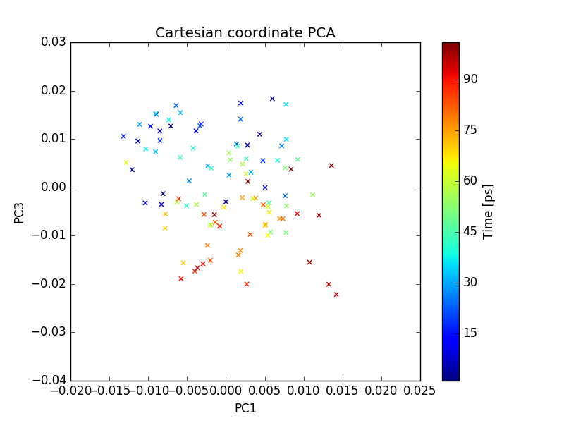
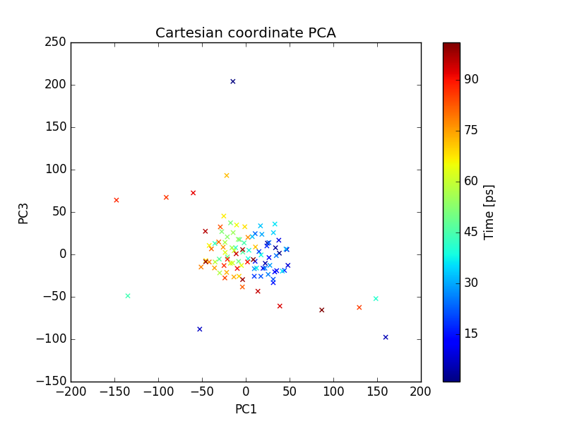
plot of PC1 and PC3
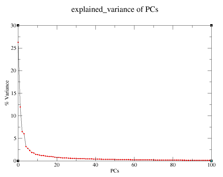
Explained variance of PCs
3.3. PCA on internal coordinates
One can also do PCA on internal coordinates of a MD trajectory. Options are available for different types of internal coordinates such as, pairwise distance between atoms, 1-3 angle between backbone atoms, phi angle, and psi angle. Run the following command to do PCA on pairwise distance between CA atoms.
internal_pca.py -t Tutorial/md_01_noWAT.xtc -p Tutorial/complex.pdb -ag CA -ct distance
Run the following command to do PCA on backbone psi angles.
internal_pca.py -t Tutorial/md_01_noWAT.xtc -p Tutorial/complex.pdb -ag CA -ct psi
Output files include 2D plot of first 3 PCs and Scree plot, which can be visualized using xmgrace as described earlier.
MDS (Multi-dimensional scaling) on a MD trajectory
To perform the MDS on pairwise RMSD between C-alpha atoms, run the following command.
mds.py -t Tutorial/md_01_noWAT.xtc -p Tutorial/complex.pdb -ag CA -dt rmsd
Output files include 2D plot of first three PCs which can be visualized using xmgrace as described earlier.
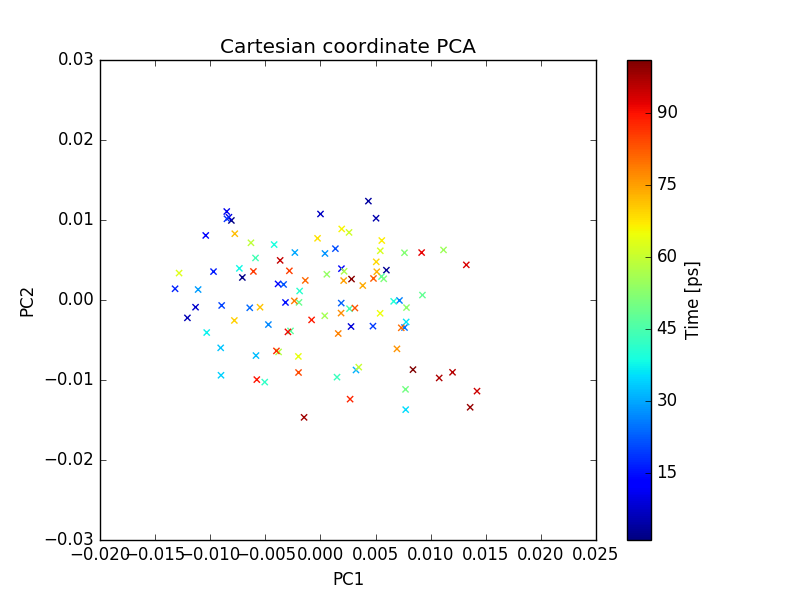
plot of PC1 and PC2
plot of PC1 and PC3
t-SNE on a MD trajectory
Run the following command to perform t-SNE using pairwise RMSD of CA atoms as the index of dissimilarity.
tsne.py -t Tutorial/md_01_noWAT.xtc -p Tutorial/complex.pdb -ag CA -dt rmsd
Output files include 2D plot of the first 3 PCs, which can be visualize using xmgrace as described earlier.
Note: The t-SNE algorithm is non-linear and highly flexible, which makes it difficult to interpret the results. Different set of parameters gives very different output. Users are required to try different set of values for “perplexity” , “learning rates”, and “number of iteration”. A useful discussion covering these issues can be found here https://distill.pub/2016/misread-tsne/
plot of PC1 and PC2
plot of PC1 and PC3